From cells to pathways: A spatial transcriptomics workflow.
Summary
Spatial transcriptomics allows researchers to measure gene activity (gene expression) while preserving the physical coordinates of the tissue (1). This is critical in cancer, where cellular context and local interactions shape disease progression. Here, I analysed a 10x Genomics Visium HD 3′ dataset (fresh frozen ovarian cancer, 8 µm binning)(2). Preprocessing was performed with Space Ranger 4, and downstream analysis used R/Seurat v5 with additional enrichment and correlation packages. The analysis pursued five goals:
- Identify the major cell types
- Distinguish tumour from non-tumour tissue
- Perform differential expression (DE)
- Run Gene Ontology (GO) and KEGG pathway enrichment
- Investigate correlations among genes and clusters.
Eight clusters were identified and mapped to epithelial, fibroblast, endothelial, and immune cell types. About 20% of spots were classified as tumour by a tumour-signature scoring scheme. Globally, 265 genes were significantly different between tumour and non-tumour regions, including strong downregulation of collagen genes (COL1A1, COL3A1, COL1A2) and actin-related genes (ACTA2, TAGLN) in tumour. Enrichment analyses highlighted extracellular matrix remodelling, cell adhesion, and signalling pathways. Correlation networks revealed 11 co-expression modules with 29 high-confidence edges, supporting functional coupling among tumour-associated markers. This study demonstrates that high-definition spatial transcriptomics can simultaneously resolve tissue composition, tumour boundaries, gene-level changes, and functional pathways, providing a multidimensional view of ovarian cancer biology.
Introduction
Spatial transcriptomics
Spatial transcriptomics is a technique that measures which genes are expressed in a tissue while also recording the exact position of each measurement (1). Think of it as combining a map with a gene expression profile: not only do we know what is happening, but also where. This makes it different from standard single-cell RNA sequencing, where cells are first dissociated from the tissue. While single-cell methods reveal detailed expression per cell, they lose the spatial arrangement, the very architecture that often defines how cells behave and interact. In cancer biology, spatial context is particularly crucial because tumour cells do not exist in isolation: they interact with surrounding fibroblasts, endothelial cells, and immune cells to form a complex micro-environment (3).
About the dataset
Ovarian cancer is one of the deadliest gynaecological malignancies, partly because it is often diagnosed late and displays a highly heterogeneous tissue structure (4). Tumour cells interact with healthy epithelial tissue, fibroblasts that produce extracellular matrix, endothelial cells that form blood vessels, and immune cells that infiltrate the tumour. Traditional gene expression profiling averages signals across these components, making it difficult to pinpoint which processes belong to which compartment. By preserving the tissue architecture, spatial transcriptomics provides a way to dissect this heterogeneity and better understand the tumour micro-environment. (5) For this project, I analysed a publicly available dataset provided by 10x Genomics, which was generated using the Visium HD 3′ assay on a fresh frozen ovarian cancer section. Visium HD offers high spatial resolution. The gene expression can be binned into 2, 8, or 16 µm squares. This high-definition capability makes it possible to approximate single-cell or even subcellular resolution. I selected the 8 µm resolution, which strikes a balance between resolution and manageable data size. Processing the data The raw sequencing files (FASTQ) and tissue images (H&E stained) were processed using Space Ranger 4, the standard software pipeline provided by 10x Genomics. This pipeline performs several key tasks:
- Read alignment: sequencing reads are mapped to the human reference genome.
- UMI counting: unique molecular identifiers (UMIs) are used to remove PCR duplicates and quantify gene expression accurately.
- Image registration: the spatial coordinates of each bin are aligned with the histological H&E image.
- HD binning: expression is aggregated into bins of 2, 8, or 16 µm.
- Segmentation: cell boundaries can be estimated from the H&E image, enabling per-cell analysis instead of fixed bins.
- The outputs include filtered count matrices (filtered_feature_bc_matrix.h5 with spatial metadata), segmentation files, QC reports (web_summary.html, metrics_summary.csv), and visualization files (.cloupe).
Goal of analysis
For this analysis, I worked with the binned 8 µm matrix together with the spatial image data. Spatial analysis produces a massive amount of information, so clear goals are essential. In this project, I focused on five objectives:
- Identify the major cell types in the tissue (epithelial, fibroblast, endothelial, immune).
- Classify tumour vs. non-tumour regions using a tumour-signature scoring system.
- Detect differentially expressed (DE) genes between tumour and non-tumour regions.
- Perform Gene Ontology (GO) and Kyoto Encyclopedia of Genes and Genomes (KEGG) pathway enrichment to see which biological processes and pathways are involved.
- Explore correlations among genes and clusters to detect co-expression modules. The analysis was carried out in R, using the Seurat v5 framework for spatial transcriptomics, together with visualization and enrichment packages such as ggplot2 and cluster Profiler. R was chosen because of its strong integration of spatial workflows, DE testing, and enrichment tools in a single ecosystem.
Methods
We analysed the public 10x Genomics Visium HD ovarian cancer dataset (fresh frozen, 3′ assay). Raw FASTQ files and histology images were processed with Space Ranger v4 for read alignment, UMI counting, image registration, and binning (see 10x Genomics documentation). We focused on the 8 µm resolution outputs.
Quality control and filtering
We processed the dataset with Space Ranger v4 and imported the 8 µm outputs into Seurat v5 (documentation). Spot-level QC metrics (total counts, detected genes, mitochondrial fraction) were inspected, and bins with <50 genes or >10% mitochondrial reads were excluded. QC summaries confirmed that filtering improved data quality without bias. The cleaned dataset was saved for downstream analyses (Script A).
Clustering and fine-tuning
Normalized and scaled data were reduced by PCA and embedded with UMAP. Using a nearest-neighbor graph, clustering was performed across a range of resolutions. A grid search evaluated silhouette scores and UMAP stability, leading to the choice of resolution 0.2, yielding eight clusters (Script B). These clusters provided the framework for annotation (Goal 1) and tumor classification (Goal 2).
Cell type annotation and tumor classification
Clusters were annotated with canonical markers: EPCAM/KRTs (epithelial, (6)), COL1A1/ACTA2 (fibroblasts,(7)), PECAM1/VWF (endothelial, (8)), PTPRC/CD3D (immune, (9, 10)). Tumor identity was assigned using a score based on PAX8, MUC16, WFDC2, and MSLN, with the 80th percentile as cutoff. Tumor spots localized to compact patches overlapping the H&E-defined tumor core (Script C).
Differential expression analysis & enrichment
Global and cell-type–specific comparisons between tumor and non-tumor spots were performed with Seurat’s Wilcoxon test, requiring a minimum detection fraction and log-fold change. Significant genes were tested for functional enrichment with clusterProfiler using GO (BP, MF, CC) and KEGG categories ((Script D) and (Script E)).
Correlation analyses
Spearman correlations among variable genes revealed co-expression modules, and cluster–cluster correlations highlighted transcriptional relationships across cell types. Heatmaps and networks were generated to visualize these structures (Script F).
This analyse add another dimension to the study. Instead of simply labeling spots or listing differentially expressed genes, correlation networks highlight the functional wiring of the tissue: which genes tend to be switched on together, and which cell compartments are most tightly linked at the transcriptomic level. Correlation analyses directly addressed Goal 5 (explore correlations among genes and clusters). It also reinforced insights from earlier steps: the modules confirmed that tumor markers co-express as a coherent program.
Results
Quality control
The raw 10x Visium HD dataset contained several hundred thousand 8 µm bins. After filtering based on detected genes, total counts, and mitochondrial content, 327,576 spots (82% of the raw dataset) remained. Retained spots had a median of 182 transcripts and 158 genes, with counts ranging from 50 to over 5,200 genes per spot. Filtering removed low-quality bins mostly at tissue edges or damaged slide regions, while preserving central tissue domains. Summary statistics are listed in table 1 and table 2.
Table 1: Best choice of QC
| Minimum features | Minimum counts | Maximum mt | Spots | Retention | Median counts | Median features | Q95 mt | Retentionscore | Feature norm | mt_inv | score |
|---|---|---|---|---|---|---|---|---|---|---|---|
| 50 | 0 | 10 | 327576 | 0.7256 | 182 | 158 | 5.305 | 1 | 0 | 1 | 0.6 |
Table 2: QC summary
| Stage | Spots | Median Counts | Median features | Q95 mt | retention |
|---|---|---|---|---|---|
| Before | 451466 | 132 | 117 | 6.944 | NA |
| After | 327576 | 182 | 158 | 5.305 | 0.7256 |
In table 1 each row represents one tested combination of thresholds for spot quality. The columns min_features, min_counts, and max_percent_mt record the exact rules used: the minimum number of genes a spot must contain, the minimum total counts required, and the maximum fraction of mitochondrial reads allowed. For each combination, the table reports how many spots remain after applying these filters (spots_retained) and what proportion of the original dataset this represents (pct_retained). To give a sense of the resulting dataset, median values are also provided for the number of transcripts per spot (median_counts) and the number of detected genes (median_features). A column marks the “best” choice, indicating which threshold combination was selected as the optimal balance between stringency and tissue coverage.
In table 2 the dataset before and after the chosen filters were applied is compared. It lists the total number of spots initially present (n_spots_before) and the number that remained after QC (n_spots_after). It also records the median transcript counts and gene features per spot in both cases (median_counts_before vs. median_counts_after; median_features_before vs. median_features_after), as well as the mean mitochondrial fraction (mean_percent_mt_before and mean_percent_mt_after). By contrasting these before-and-after statistics, the table makes clear how much data was removed, how quality improved, and how representative the retained spots are.
Clustering
To explore transcriptional structure, I tested multiple clustering settings in a grid search. Varying principal components (12, 15, 20), neighbourhood sizes (10, 15, 20), and resolutions (0.2–1.0) produced between 7 and 14 clusters depending on parameters. Higher resolutions (≥0.8) split the dataset into many small clusters (<2% of spots each) that lacked stability. Lower resolutions (0.2–0.4) produced 7–8 clusters, each representing 5–23% of spots. Silhouette scores indicated better separation at lower resolutions. A snippet of grid search outcomes is provided in table 3. Each row in table 3 represents one tested parameter combination. The columns pcs, k, and resolution record the specific settings: the number of principal components used for dimensionality reduction, the neighborhood size (k) considered when constructing the graph for clustering, and the resolution parameter that controls how finely or coarsely the data are partitioned. For each combination, the file reports how many clusters were produced (n_clusters), allowing direct comparison of how parameter choices affect the granularity of the results.
To evaluate cluster quality, table 3 also includes several summary statistics. silhouette_score measures how well separated the clusters are: higher values indicate that spots are more similar within clusters and more distinct between clusters. avg_cluster_size gives the mean number of spots per cluster, while min_cluster_size and max_cluster_size record the extremes. These metrics help identify settings that avoid both fragmentation into many tiny clusters and collapse into overly broad groups. pct_small_clusters indicates the proportion of clusters that fall below a given minimum size threshold, highlighting parameter choices that produce biologically less interpretable results.
Table 3: Fine-tune grid search
| pcs | k | res | n_clusters | frac_small | sil_median | penalty_n | rank_sil | rank_pen | rank_small | rank_sum |
|---|---|---|---|---|---|---|---|---|---|---|
| 12 | 10 | 0.2 | 8 | 0 | 0.0216241784241777 | 0 | -44 | 15 | 17.5 | -11.5 |
| 12 | 10 | 0.4 | 15 | 0 | -0.0594859710793455 | 0 | -25 | 15 | 17.5 | 7.5 |
| 12 | 10 | 0.6 | 21 | 0 | -0.0523806929207793 | 1 | -31 | 30 | 17.5 | 16.5 |
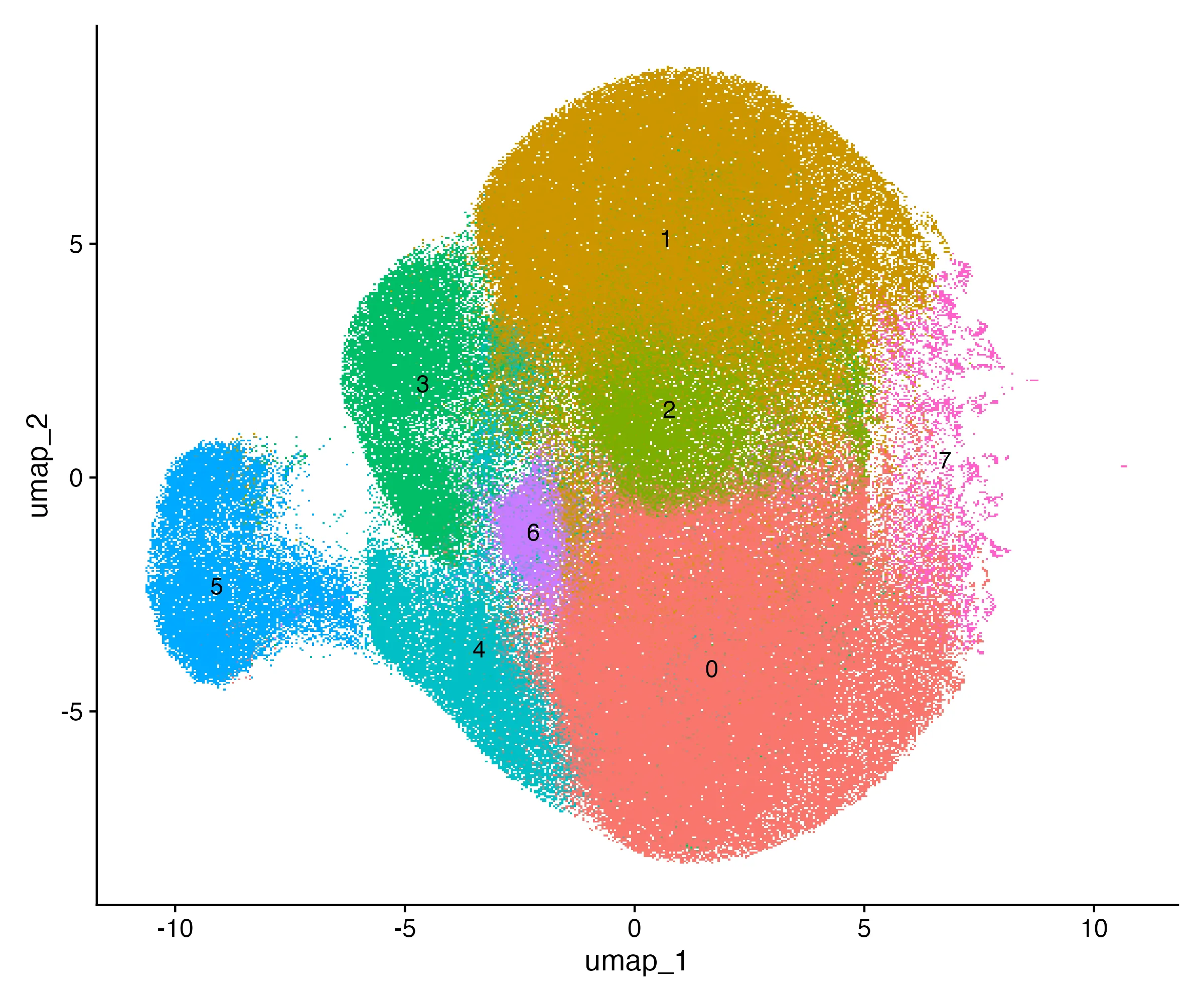
I selected resolution 0.2, which yielded 8 clusters. Cluster sizes ranged from 12,000 spots (4%) to 74,000 spots (23%). The UMAP embedding showed eight well-separated groups (Figure 1).
Cell type annotation
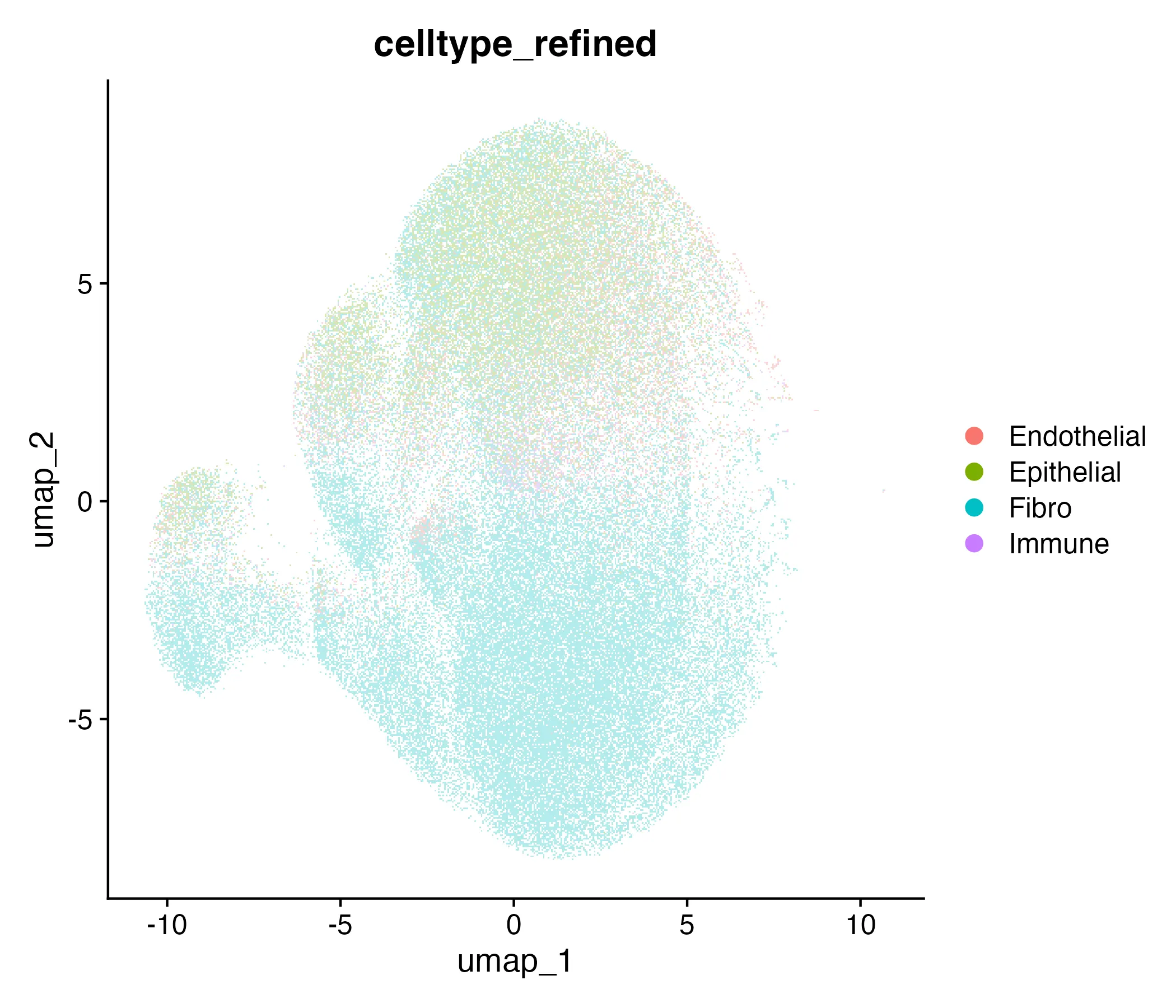
Each cluster was annotated by marker gene expression. The mapping resulted in four major categories: • Epithelial (Clusters 1 & 4, ~38% of spots): EPCAM, KRT8, KRT18. • Fibroblast (Clusters 2, 3 & 7, ~34% of spots): COL1A1, COL1A2, ACTA2, TAGLN. • Endothelial (Cluster 6, ~10% of spots): PECAM1, VWF, KDR. • Immune (Clusters 5 & 8, ~18% of spots): PTPRC, CD3D, MS4A1, NKG7.
For example, Cluster 3 (42,000 spots, 13%) expressed COL1A1 and ACTA2, consistent with fibroblasts, while Cluster 1 (61,000 spots, 19%) expressed EPCAM and KRT8, typical of epithelial cells. Table 4 shows that each transcriptional cluster was assigned to a biological cell type. the column celltype records the chosen biological identity, such as “Epithelial,” “Fibro,” “Endothelial,” or “Immune.”
Table 4: Cluster annotation by cell type
| cluster | celltype |
|---|---|
| 0 | Fibro |
| 1 | Fibro |
| 2 | Fibro |
| 3 | Fibro |
| 4 | Fibro |
| 5 | Fibro |
| 6 | Fibro |
| 7 | Fibro |
The UMAP colored by cell type and the corresponding spatial map are shown in Figure 2.
Tumor classification
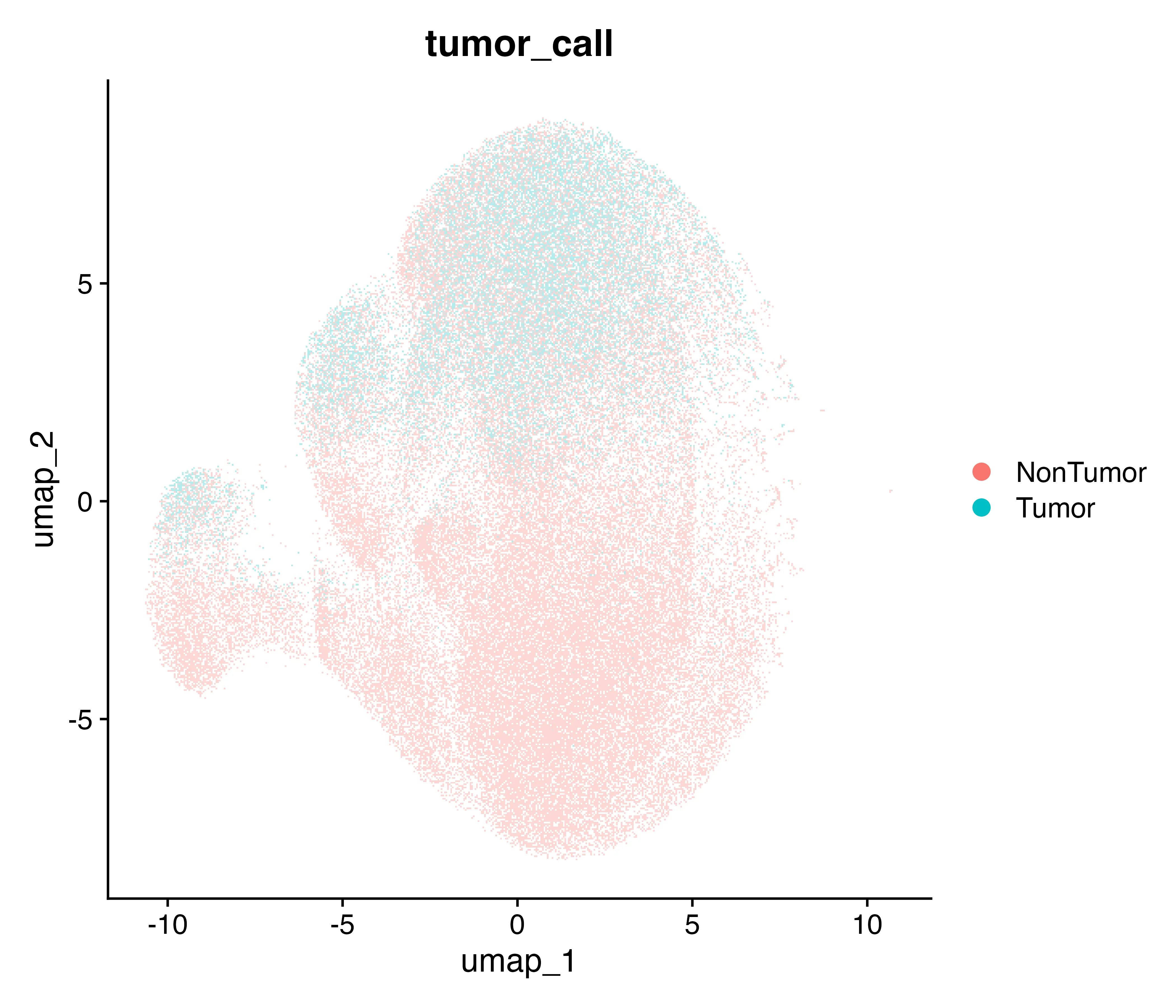
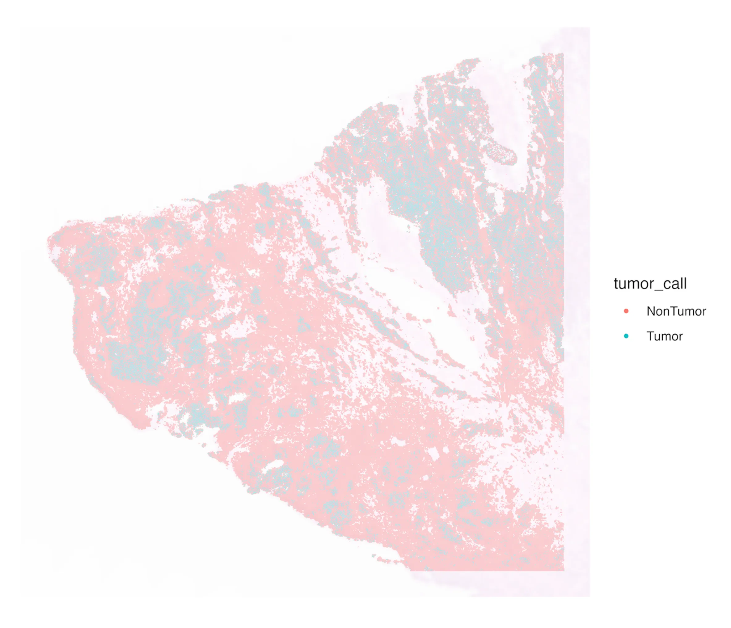
To identify tumor regions, I calculated a tumor score per spot using markers (PAX8, MUC16, WFDC2, MSLN). Scores ranged from –1.1 to +2.4, with a clear shift at the 80th percentile (–0.0206). Spots above this cutoff were labeled tumor. This yielded 65,500 tumor spots (20% of all retained spots). Tumor spots clustered in contiguous regions that overlapped with epithelial-rich domains, while non-tumor spots aligned with fibroblast, endothelial, and immune areas. The UMAP projection and spatial tumor map are shown in Figure 3.
Differential expression
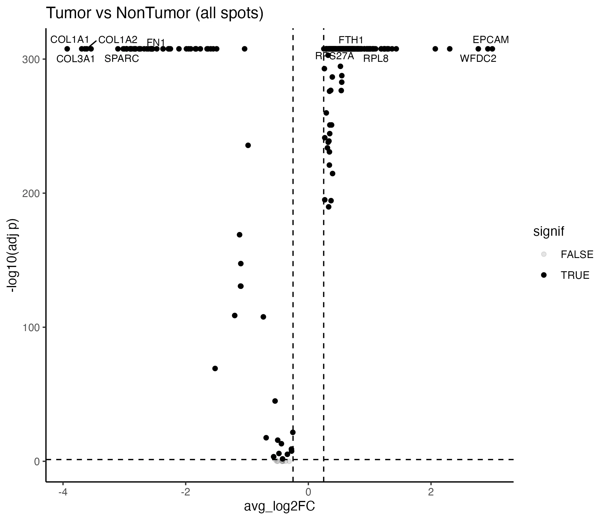
Comparing tumor versus non-tumor spots identified 265 significant genes (adjusted p < 0.05), of which 194 were upregulated and 71 downregulated in tumor. The strongest downregulated genes were COL1A1 (log2FC –3.93), COL3A1 (–3.70), ACTA2 (–3.64), COL1A2 (–3.61), and TAGLN (–3.54) (Table 1 in (Appendix). Cell-type–specific contrasts revealed variable scales of change:
- Endothelial: 31 genes (28 up, 3 down),
- Epithelial: 22 genes (9 up, 13 down),
- Fibroblast: 257 genes (187 up, 70 down),
- Immune: 24 genes (20 up, 4 down).
Top hits included WFDC2, MSLN, MUC16 in endothelial cells, KRT8, EPCAM, KRT18 in epithelial cells, and APOE downregulated in immune cells (Table 2, Appendix). The global volcano plot is shown in Figure 4, with additional volcano plots per cell type in Appendix as Figure 1 through 4.
Functional enrichment
GO and KEGG enrichment linked differential expression to functional processes. Top GO Biological Processes included extracellular matrix organization, cytoskeletal organization, and cell adhesion. Molecular Functions were dominated by structural molecule activity and actin binding, while Cellular Components included focal adhesion and basement membrane.
KEGG pathways enriched in tumor-associated genes included ECM–receptor interaction, PI3K–Akt signaling, and focal adhesion. The top 3 functions per cluster are represented in table 3. The top three for GO and also for KEGG are represented.
Table 3: Top 3 functions per cluster.
| cluster | GO_BP_top3 | GO_MF_top3 | GO_CC_top3 | KEGG_top3 |
|---|---|---|---|---|
| 0 | extracellular matrix organization | endodermal cell differentiation | cell-substrate adhesion | extracellular matrix structural constituent | collagen binding | glycosaminoglycan binding | collagen-containing extracellular matrix | endoplasmic reticulum lumen | collagen trimer | Cytoskeleton in muscle cells | ECM-receptor interaction | Focal adhesion |
| 1 | cytoplasmic translation | ribosomal small subunit biogenesis | aerobic electron transport chain | structural constituent of ribosome | oxidoreduction-driven active transmembrane transporter activity | rRNA binding | cytosolic ribosome | focal adhesion | small-subunit processome | Coronavirus disease - COVID-19 | Oxidative phosphorylation | Diabetic cardiomyopathy |
| 2 | cytoplasmic translation | humoral immune response | antimicrobial humoral response | structural constituent of ribosome | peptide antigen binding | protein tag activity | cytosolic ribosome | phagocytic vesicle | small-subunit processome | Coronavirus disease - COVID-19 | Antigen processing and presentation | Phagosome |
| 3 | collagen fibril organization | transforming growth factor beta production | cellular response to amino acid stimulus | extracellular matrix structural constituent | collagen binding | protease binding | collagen-containing extracellular matrix | collagen trimer | endoplasmic reticulum lumen | Cytoskeleton in muscle cells | Proteoglycans in cancer | ECM-receptor interaction |
| 4 | antigen processing and presentation of exogenous peptide antigen | peptide antigen assembly with MHC protein complex | regulation of immune effector process | peptide binding | MHC class II protein complex binding | antigen binding | MHC protein complex | lumenal side of endoplasmic reticulum membrane | ER to Golgi transport vesicle membrane | Antigen processing and presentation | Phagosome | Allograft rejection |
| 5 | B cell receptor signaling pathway | antibacterial humoral response | regulation of respiratory burst | antigen binding | immunoglobulin receptor binding | glycosaminoglycan binding | blood microparticle | immunoglobulin complex | immunoglobulin complex, circulating | Cytoskeleton in muscle cells |
| 6 | integrin-mediated signaling pathway | extracellular matrix organization | endodermal cell differentiation | extracellular matrix structural constituent | collagen binding | growth factor binding | collagen-containing extracellular matrix | endoplasmic reticulum lumen | focal adhesion | Focal adhesion | ECM-receptor interaction | Cytoskeleton in muscle cells |
| 7 | cytoplasmic translation | ribosome biogenesis | positive regulation of nuclear-transcribed mRNA catabolic process, deadenylation-dependent decay | structural constituent of ribosome | mRNA binding | translation factor activity, RNA binding | cytosolic ribosome | rough endoplasmic reticulum | focal adhesion | Coronavirus disease - COVID-19 |
Correlation analysis
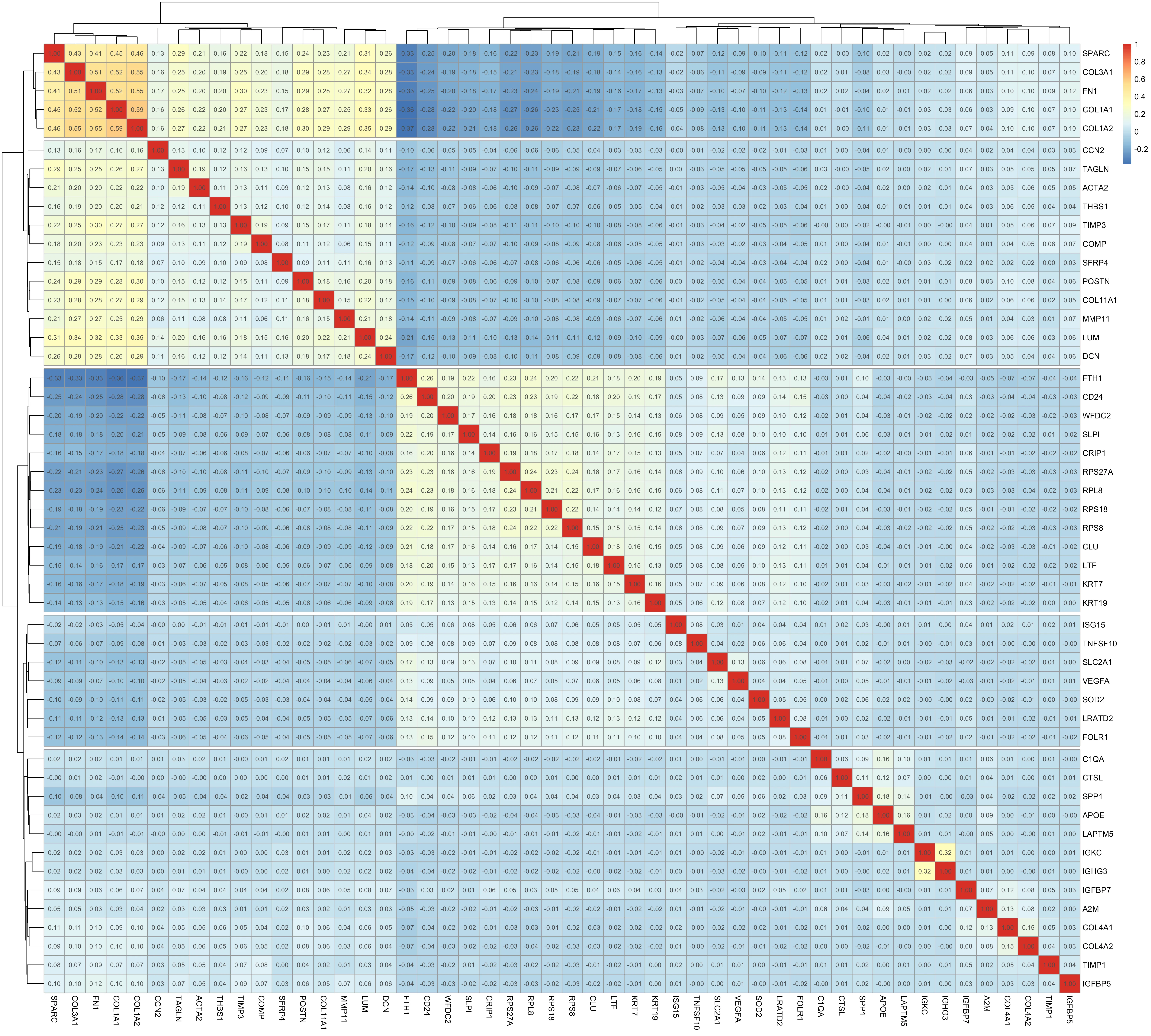
Correlation analysis of ~1,500 highly variable genes across ~80,000 sampled spots yielded 29 significant edges forming 11 modules. Modules ranged from 4 to 25 genes. Epithelial modules included EPCAM, KRT8, KRT18; fibroblast modules centered on collagens (COL1A1, COL3A1); and immune modules contained PTPRC and CD3D.
Cluster–cluster correlations confirmed strong similarity among epithelial tumor clusters and distinct profiles for fibroblast and immune clusters. To investigate co-expression patterns, we performed correlation analyses at both the gene and cluster level. The gene–gene correlation heatmap (Figure 5) revealed 11 modules comprising 29 significant edges. One of the largest modules contained collagens (COL1A1, COL1A2, COL3A1) together with ACTA2 and TAGLN, reflecting fibroblast activity and extracellular matrix remodeling. Another module grouped epithelial markers (EPCAM, KRT8, KRT18) into a coherent block, while immune-associated genes such as PTPRC and CD3D clustered separately. These modules highlight transcriptional programs that recur across spatial domains of the tissue.
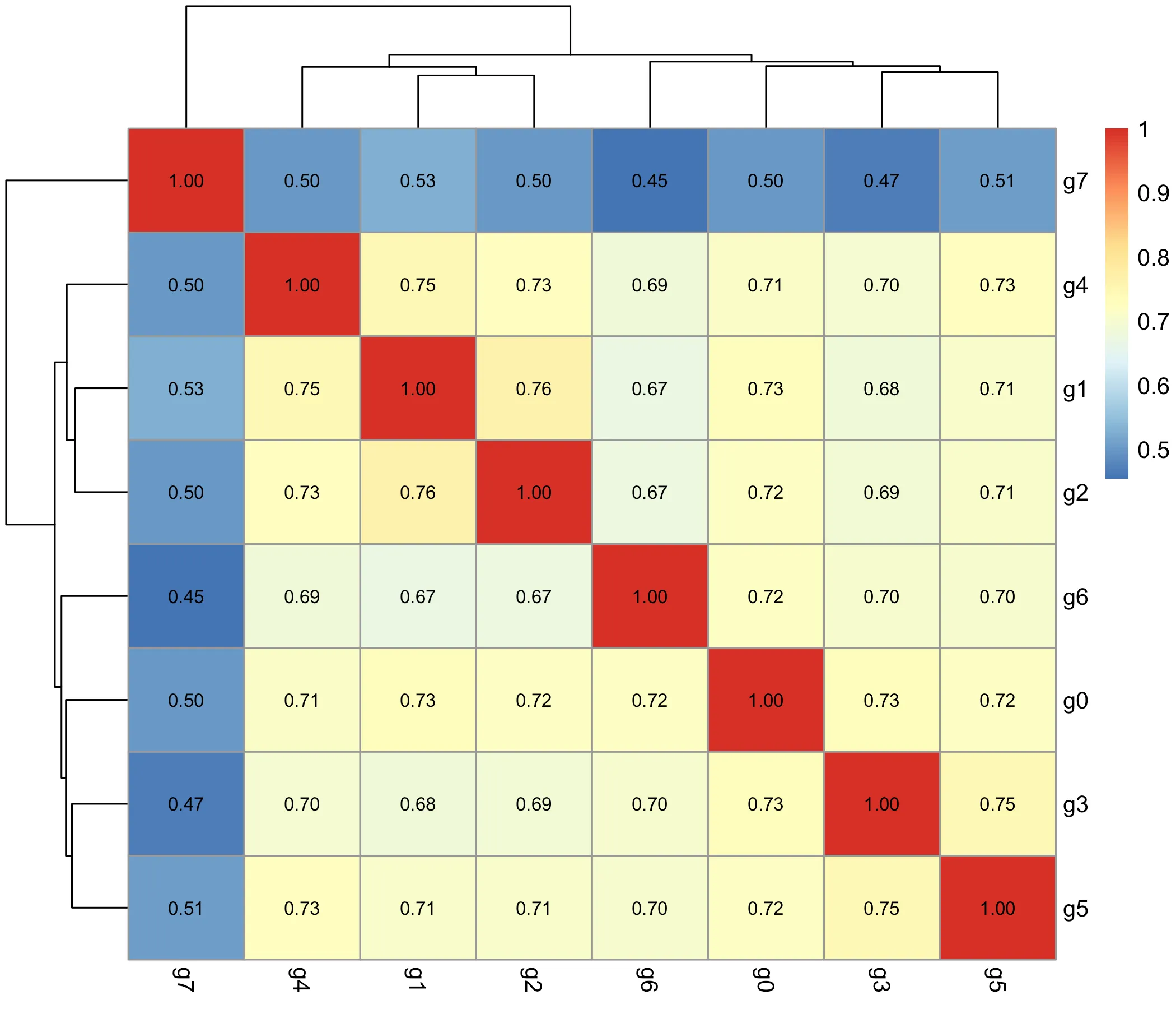
At the cluster level, the correlation heatmap (Figure 6) showed clear structure. The two epithelial tumor clusters (g1, g2) were highly correlated, indicating similar expression programs across distinct tumor regions. Fibroblast clusters (g3, g4, g7) formed their own correlated group, consistent with their shared extracellular matrix signatures. Immune (g5) and endothelial (g6) clusters remained distinct, correlating only modestly with other groups. This analysis demonstrates that both gene-level and cluster-level correlation patterns converge on biologically meaningful modules, reinforcing the robustness of the earlier cell-type annotations.
Discussion
This study applied high-definition spatial transcriptomics to ovarian cancer tissue using the 10x Genomics Visium HD platform. Through an integrated pipeline, covering quality control, clustering, cell-type annotation, tumor calling, differential expression, enrichment, and correlation analysis, we generated a spatially resolved molecular map of the tumor and its microenvironment.
Key findings
The analysis retained 327,576 high-quality spots, which grouped into eight stable clusters. These clusters corresponded to four major cell categories (epithelial, fibroblast, endothelial, immune) and showed clear alignment with tissue structure. Approximately 20% of spots (≈65,500) were classified as tumor, forming compact domains that overlapped with histological tumor cores. A global tumor–non-tumor comparison revealed 265 differentially expressed genes, dominated by downregulation of structural and cytoskeletal genes such as COL1A1, COL3A1, ACTA2, COL1A2, and TAGLN. Enrichment analysis highlighted extracellular matrix organization, adhesion, and PI3K–Akt signaling, while correlation analysis identified 11 co-expression modules (29 high-confidence edges) that grouped epithelial, fibroblast, and immune programs. Together, these results form a coherent view of ovarian cancer architecture at high spatial resolution.
Comparison with prior work
These findings align with established features of ovarian cancer biology. The recovery of tumor markers such as PAX8, MUC16 (CA125), WFDC2 (HE4), and MSLN (mesothelin) is consistent with their recognized clinical roles in diagnosis and monitoring (12-14). The strong downregulation of collagens and actin-associated genes reflects stromal remodeling by cancer-associated fibroblasts, a process widely described in solid tumors (15). Importantly, by preserving tissue context, spatial transcriptomics captures these processes in situ, something that single-cell RNA-seq cannot, as it relies on dissociation (16). In this way, our results confirm both the expected biology and the added value of spatial approaches.
Consistency across analyses
Different layers of the workflow converged on the same biological signals. Clustering and annotation produced interpretable groups that matched known marker panels. Tumor scoring at the 80th percentile yielded spatial domains that mirrored histology. Differential expression highlighted extracellular matrix genes, which were also dominant in GO and KEGG enrichment. Correlation analysis further grouped these genes into fibroblast modules, reinforcing the same theme from another angle. This triangulation across clustering, tumor classification, DE, enrichment, and correlation strengthens confidence in the results. Minor discrepancies were present: for example, epithelial clusters showed only 22 significant genes, compared to 257 in fibroblasts. This imbalance may reflect the mixed nature of 8-µm bins, lower coverage in epithelial regions, or genuine heterogeneity. Such differences highlight both the value and the limitations of the current resolution.
Technical considerations
Several technical choices shaped the analysis. The use of 8-µm bins increased resolution compared to classic Visium but still combined signals from neighboring cells, especially at compartment boundaries (17). Tumor classification was based on a percentile cutoff using signature genes, which is transparent and reproducible but inevitably subjective. Alternative approaches such as CNV-based inference (e.g., inferCNV, copyKAT) or reference mapping could increase specificity (18). For differential expression, a Wilcoxon rank-sum test with Benjamini–Hochberg correction was applied, a common choice in single-cell and spatial analysis (19-20). Nonetheless, results remain sensitive to compositional differences between tumor and non-tumor groups. Together, these considerations show that while the pipeline is robust, its precision depends on methodological parameters.
Limitations
This study also has limitations. First, bin resolution remains below true single-cell level, introducing mixing of adjacent signals. Second, marker-based annotation introduces reference bias, since panels are curated from literature and may overlook less characterized populations. Third, tumor scoring relied on a simple cutoff, which could miss borderline cases. Finally, the dataset analyzed here represents a single sample, limiting generalizability across patients and subtypes. These limitations should be viewed as opportunities for refinement rather than weaknesses, as they point to concrete areas for future methodological development.
Future directions
Future work can improve on several fronts. Moving toward cell-segmented outputs will reduce signal mixing and sharpen boundaries between cell types (21). Incorporating CNV-like inference alongside expression-based scoring may yield more specific tumor calls (18). Expanding to multi-sample or cohort-level datasets would allow replication and capture inter-patient variability. Beyond R, Python frameworksoffer compelling options for post-processing: Scanpy for scalable analysis (22), Squidpy for histology-aware features (23), and scvi-tools for probabilistic models (24)](#References). Integration with imaging libraries such as MONAI could link transcriptomic data to digital pathology. Finally, packaging the workflow in Snakemake or Nextflow would enhance reproducibility and make it easier to share (25-26). These directions illustrate how current limitations can evolve into strengths as the field advances.
Closing perspective
In sum, this study shows that high-definition spatial transcriptomics can deliver a consistent and interpretable view of ovarian cancer biology. By combining clustering, annotation, tumor delineation, differential expression, enrichment, and correlation analysis, the workflow mapped both cellular composition and molecular programs. With refinements in resolution, tumor calling, and multi-sample integration, and by extending into Python-based ecosystems for advanced post-processing, such pipelines will become even more powerful. This balance of strengths, limitations, and future opportunities highlights the promise of spatial transcriptomics for unraveling tumor architecture and guiding more precise research in oncology.
Acknowledgements
We acknowledge 10x Genomics for providing the public dataset and the developers of Scanpy and Squidpy for the open-source tools that made this analysis possible.
References:
- Tian, L., Chen, F., & Macosko, E. Z. (2023). The expanding vistas of spatial transcriptomics. Nature Biotechnology, 41(6), 773-782.
- Visium HD 3’ Gene Expression Library, Ovarian Cancer (Fresh Frozen) | 10x Genomics. (n.d.). https://www.10xgenomics.com/datasets/visium-hd-three-prime-ovarian-cancer-fresh-frozen6
- Long, J. A. (2015). Quantifying spatial-temporal interactions from wildlife tracking data: Issues of space, time, and statistical significance. Procedia Environmental Sciences, 26, 3–10.
- Jayson, G. C., Kohn, E. C., Kitchener, H. C., & Ledermann, J. A. (2014). Ovarian cancer. The lancet, 384(9951), 1376-1388.
- Ungefroren, H., Sebens, S., Seidl, D., Lehnert, H., & Hass, R. (2011). Interaction of tumor cells with the microenvironment. Cell Communication and Signaling, 9(1), 18.
- Trzpis, M., McLaughlin, P. M., De Leij, L. M., & Harmsen, M. C. (2007). Epithelial cell adhesion molecule: more than a carcinoma marker and adhesion molecule. The American journal of pathology, 171(2), 386-395.
- LeBleu, V. S., & Kalluri, R. (2018). A peek into cancer-associated fibroblasts: origins, functions and translational impact. Disease models & mechanisms, 11(4), dmm029447.
- Müller, A. M., Hermanns, M. I., Skrzynski, C., Nesslinger, M., Müller, K. M., & Kirkpatrick, C. J. (2002). Expression of the endothelial markers PECAM-1, vWf, and CD34 in vivo and in vitro. Experimental and molecular pathology, 72(3), 221-229.
- Al Barashdi, M. A., Ali, A., McMullin, M. F., & Mills, K. (2021). Protein tyrosine phosphatase receptor type C (PTPRC or CD45). Journal of clinical pathology, 74(9), 548-552.
- Li, Q., Yang, Z., Ling, X., Ye, J., Wu, J., Wang, Y., … & Zheng, J. (2023). Correlation Analysis of Prognostic Gene Expression, Tumor Microenvironment, and Tumor‐Infiltrating Immune Cells in Ovarian Cancer. Disease Markers, 2023(1), 9672158.
- Muinao, T., Boruah, H. P. D., & Pal, M. (2019). Multi-biomarker panel signature as the key to diagnosis of ovarian cancer. Heliyon, 5(12).
- Laury, A. R., Perets, R., Piao, H., Krane, J. F., Barletta, J. A., French, C., … & Hirsch, M. S. (2011). A comprehensive analysis of PAX8 expression in human epithelial tumors. The American journal of surgical pathology, 35(6), 816-826.
- Bast Jr, R. C., Badgwell, D., Lu, Z., Marquez, R., Rosen, D., Liu, J., … & Lu, K. (2005). New tumor markers: CA125 and beyond. International journal of gynecological cancer, 15, 274-281.
- Hellstrom, I., Raycraft, J., Hayden-Ledbetter, M., Ledbetter, J. A., Schummer, M., McIntosh, M., … & Hellström, K. E. (2003). The HE4 (WFDC2) protein is a biomarker for ovarian carcinoma. Cancer research, 63(13), 3695-3700.
- LeBleu, V. S., & Kalluri, R. (2018). A peek into cancer-associated fibroblasts: origins, functions and translational impact. Disease models & mechanisms, 11(4), dmm029447.
- Moses, L., & Pachter, L. (2022). Museum of spatial transcriptomics. Nature methods, 19(5), 534-546.
- Visium HD 3’ Spatial Gene Expression User Guide | 10x Genomics. (n.d.). 10x Genomics. https://www.10xgenomics.com/support/spatial-gene-expression-hd-three-prime/documentation/steps/library-construction/visium-hd-3-prime-spatial-gene-expression-user-guide
- Song, M., Ma, S., Wang, G., Wang, Y., Yang, Z., Xie, B., … & Zhang, L. (2025). Benchmarking copy number aberrations inference tools using single-cell multi-omics datasets. Briefings in Bioinformatics, 26(2), bbaf076.
- Satija, R., Farrell, J. A., Gennert, D., Schier, A. F., & Regev, A. (2015). Spatial reconstruction of single-cell gene expression data. Nature biotechnology, 33(5), 495-502.
- Benjamini, Y., & Hochberg, Y. (1995). Controlling the false discovery rate: a practical and powerful approach to multiple testing. Journal of the Royal statistical society: series B (Methodological), 57(1), 289-300.
- Han, S., Phasouk, K., Zhu, J., & Fong, Y. (2024). Optimizing deep learning-based segmentation of densely packed cells using cell surface markers. BMC Medical Informatics and Decision Making, 24(1), 124.
- Wolf, F. A., Angerer, P., & Theis, F. J. (2018). SCANPY: large-scale single-cell gene expression data analysis. Genome biology, 19(1), 15.
- Palla, G., Spitzer, H., Klein, M., Fischer, D., Schaar, A. C., Kuemmerle, L. B., … & Theis, F. J. (2022). Squidpy: a scalable framework for spatial omics analysis. Nature methods, 19(2), 171-178.
- Gayoso, A., Lopez, R., Xing, G., Boyeau, P., Valiollah Pour Amiri, V., Hong, J., … & Yosef, N. (2022). A Python library for probabilistic analysis of single-cell omics data. Nature biotechnology, 40(2), 163-166.
- Mölder, F., Jablonski, K. P., Letcher, B., Hall, M. B., Tomkins-Tinch, C. H., Sochat, V., … & Köster, J. (2021). Sustainable data analysis with Snakemake. F1000Research, 10, 33.
- Di Tommaso, P., Chatzou, M., Floden, E. W., Barja, P. P., Palumbo, E., & Notredame, C. (2017). Nextflow enables reproducible computational workflows. Nature biotechnology, 35(4), 316-319.
