Genomics on AWS

Bioinformatics is not that hard.

Today I’m going to show you how to set up a bioinformatics pipeline in the AWS cloud.

I recently discovered a fantastic resource for engineers trying to dip their toes into the world of bioinformatics.

It was published in 2022 by Saint Jude’s Children Research Hospital.

It’s well worth a read. It starts by introducing a number of foundational concepts including cells, genes, chromosomes, transcription (the transfer of information from DNA to RNA) and translation (the process of protein synthesis based on RNA instructions).

It then delves into modern sequencing approaches and how genomic variations in an individual are identified. This is done by comparing their genomic data with a reference genome that represents the entire species. This process is commonly referred to as alignment.

A bioinformatics pipeline

The final section called “Worked example” is an end-to-end example of how to set up a bioinformatics pipeline based on real genomic data and using modern tooling.

I’m going to implement the worked example step by step and detail each step, giving extra context along the way.

To tackle genomic datasets, you’ll need a computer with serious CPU power and memory. But don’t worry, I’ve got your back. I’ll teach you how to harness the cloud so you can follow this tutorial on even the most basic laptop. Let’s go!

Setting up an EC2 instance on AWS

Before we start you’ll need an AWS account. You can create one for free. When you’re all set up, go to the EC2 console by typing ‘EC2’ in the search bar.

EC2 is the AWS service that lets you spin up a cloud computer on demand. Ok, we’re ready to launch your first EC2 instance on AWS.

Hit ‘Launch instance’. This will lead us to the instance configuration page. The first step is to choose the operating system. Many bioinformaticians use Ubuntu, so that’s what I’m going to go with, but you could choose Amazon Linux as well. The tutorial calls for at least an Intel i7 processor with 8 cores and at least 8GB of RAM and 60GB of free disk space.

A C6a.4xlarge instance seems like a good choice. It has 32GB of RAM, 16 cores (vCPUs) and is optimized for compute-intensive tasks.

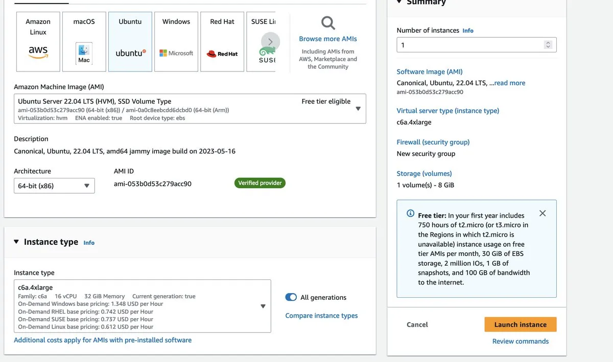
AWS will ask you to select or create a private key to manage your instance. This will be important when we SSH into it in a minute. You’ll need to make your instance accessible from your own IP address (or via a NAT Gateway).

To add persistent disk storage to your EC2 instance, simply attach a 100GB EBS volume. We want to be on the safe side, after all—EC2 needs room for the OS.

…and launch! With our instance up and running, it’s time to connect and dive into our bioinformatics pipeline.

Keep in mind that while the instance is running, it’s eating into our budget. To prevent unnecessary expenses, simply stop the instance when it’s not in use.

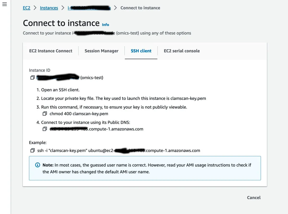
We’re going to connect to our instance using SSH.

Install bioinformatics tools

Select your new instance in the EC2 console and hit ‘Connect’. Then copy the instructions in a terminal window, using the private key that you created in the previous step.

Now that we’ve connected to our instance we can set up our environment by installing a set of bioinformatics tools (such as samtools, BWA, bcftools and FastQC).

The tutorial proposes to install everything using bioconda, a specialized conda channel for bioinformatics software packages. If you want to go this route you can install miniconda in a subdirectory of your home folder (/home/ubuntu). This runs an installer that asks for license approval and a path to install miniconda3. By installing miniconda you also install Python.

mkdir -p ~/miniconda3
wget -O ~/miniconda3/miniconda.sh https://repo.anaconda.com/miniconda/Miniconda3-latest-Linux-x86_64.sh
bash ~/miniconda3/miniconda.sh -b -u -p ~/miniconda3

You typically want to call bioconda by just typing conda command. For this you need to add miniconda to your PATH environment variable. You can do this by adding the following line to ~/.bashrc (using a text editor such as vi or nano).

# Add this line at the end of your .bashrc
export PATH=~/miniconda3/bin:$PATH

After modifying the .bashrc don’t forget to source it such that the new changes apply.

source ~/.bashrc

Before you can use conda to install all of your dependencies, you have to initialise it and configure the channels you’re going to use:

conda init bash

conda config --add channels defaults
conda config --add channels bioconda
conda config --add channels conda-forge
conda config --set channel_priority strict

You can then run conda to create your project and install the different bioinformatics packages required for the tutorial. You’ll need to run ‘conda activate’ for your dependencies to be available in your environment.

conda create -n worked-example -c bioconda bcftools==1.9 bwa==0.7.17 fastqc==0.11.8 samtools==1.9 picard==2.21.2 -y
conda activate worked-example

In my experience though, bioconda tends to hang in ‘Solving environment’ state if it thinks there are conflicts between package versions. While these can be worked around by doing atomic package installations, it’s often easier to just install each package using standard tools. For example a specific version of samtools can be installed like this:

wget https://github.com/samtools/samtools/releases/download/1.x.x/samtools-1.13.tar.bz2
tar -jxf samtools-1.13.tar.bz2
cd samtools-1.13
make

The dataset

One way or another we have our environment all set up. We have the tools now we need data. The tutorial proposes sequence data from the Thousand Genomes project, a public dataset featuring whole genome sequences of a large number of individuals.

The specific sequence that we’ll be downloading and analyzing belongs to a B lymphocyte cell line from the blood of a British female, and using an Epstein Barr Virus transformant. EBV can transform B-lymphocytes into continuously multiplying, immortal cells. As you can imagine, this is very helpful for analysis.

wget ftp://ftp.1000genomes.ebi.ac.uk/vol1/ftp/phase3/data/HG00133/sequence_read/SRR038564_{1,2}.filt.fastq.gz

After downloading the dataset, we now have two gzipped FASTQ files: SRR038564_1.filt.fastq.gz and SRR038564_2.filt.fastq.gz. FASTQ is a text-based format used to represent DNA (or RNA). It includes quality scores for each base, indicating the reliability of each base call. The FASTQ format is widely used in high-throughput sequencing, as is the case here. In this case the dataset was obtained by sequencing genetic data using an Illumina sequencer machine.

Verifying the dataset

Before we proceed with analyzing the FASTQ datasets, let’s perform some basic checks on them using the previously installed fq utility.

fq lint SRR038564_1.filt.fastq.gz SRR038564_2.filt.fastq.gz && echo 'Successfully verified FASTQs.' || echo 'Failed to verify FASTQs!'

The fq lint command operates much like a linter, ensuring the proper format of JSON or Python files. In this instance, it is used to verify the format compliance of FASTQ files.

While the results may not reveal any major surprises, they do provide valuable insights.

Notice the second line stating ‘validating paired-end reads’. This indicates that the fq tool is processing paired-end data.

In DNA sequencing, DNA is fragmented, and paired-end sequencing involves reading both ends of each fragment. Paired-end sequencing provides extended read lengths, improved mapping accuracy, and the ability to detect insertions, deletions, and rearrangements. Generally, it is more accurate (albeit more expensive) compared to single-read sequencing. The linting step also tells us that a total of 18,810,443 paired-end records were identified, and that no formatting abnormalities were found.

Generating FastQC reports

Next we’re going to generate an HTML report based on the result of the sequencing using the FastQC tool. The tutorial wants us to open the HTML file by running open SRR038564\_{1,2}.filt_fastqc.html. The open command on MacOS leads to opening a file in the computer’s default browser.

But we’re working on a remote EC2 instance that doesn’t have a browser installed. But it would be nice to see the FastQC report in our browser. So for that we’re going to publish the report on an S3 bucket and open it from there.

S3 is AWS’s cheap and reliable object storage solution. We’re going to go back to the AWS console to create a bucket.

We’re going to transfer some files from the EC2 instance to the S3 bucket and we’ll want to open them from there, so we’re going to enable public access on the bucket.

This is usually not a good practice, and we could limit the access rights, but we’ll keep it simple for now.

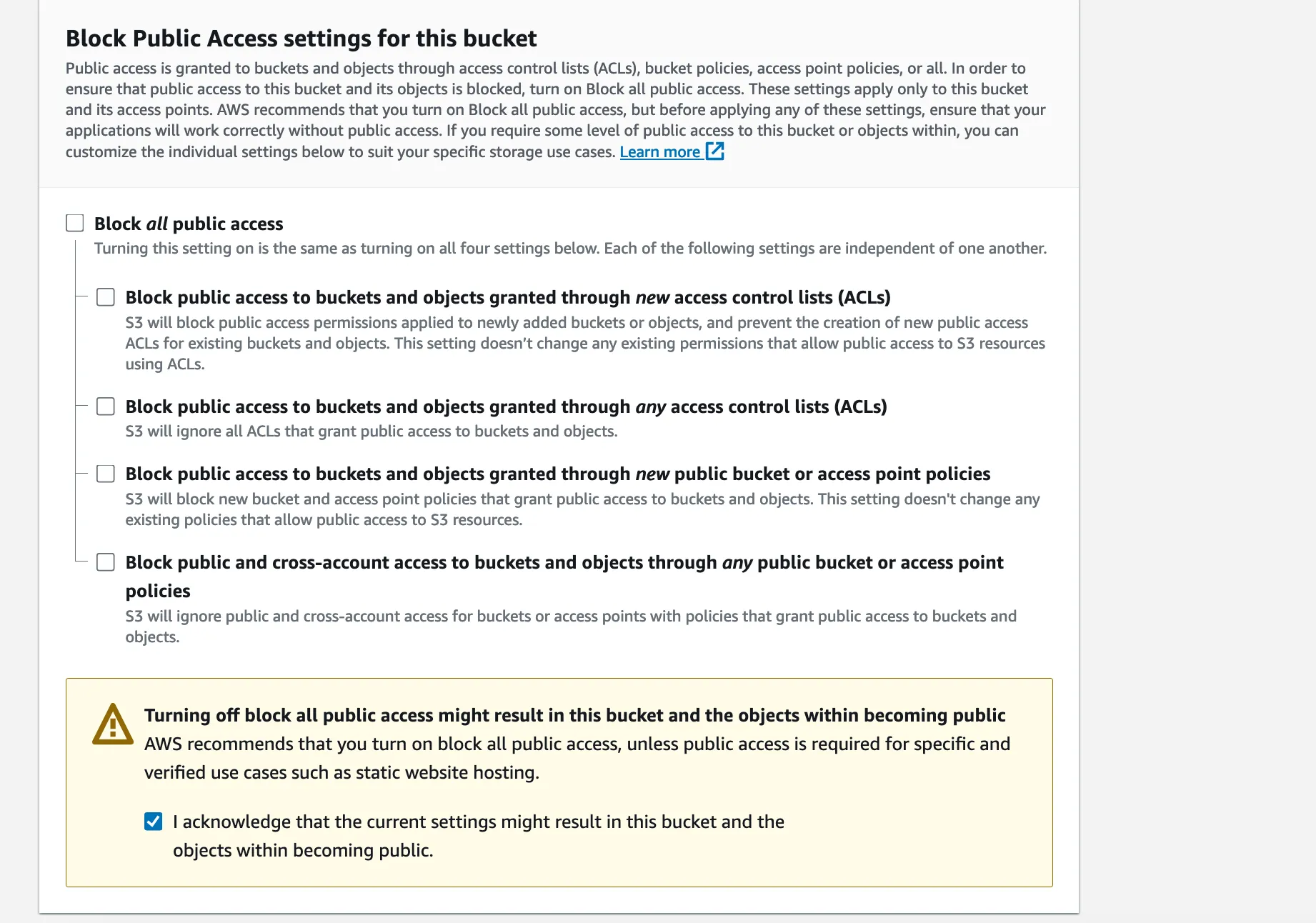
Press ‘Create bucket’ and we’re done. Now to transfer the reports over we have to grant write access to the new bucket to our EC2 instance.

For this we need to create a new IAM role for EC2 and set it as the instance profile of our EC2. IAM is AWS’s identity and access management service. It lets you set up permissions for people in your organisation, but also for servers and applications.

Let’s head over to the IAM console. We’ll have to start by defining a new IAM policy that grants permissions to write files in the S3 bucket we just created.

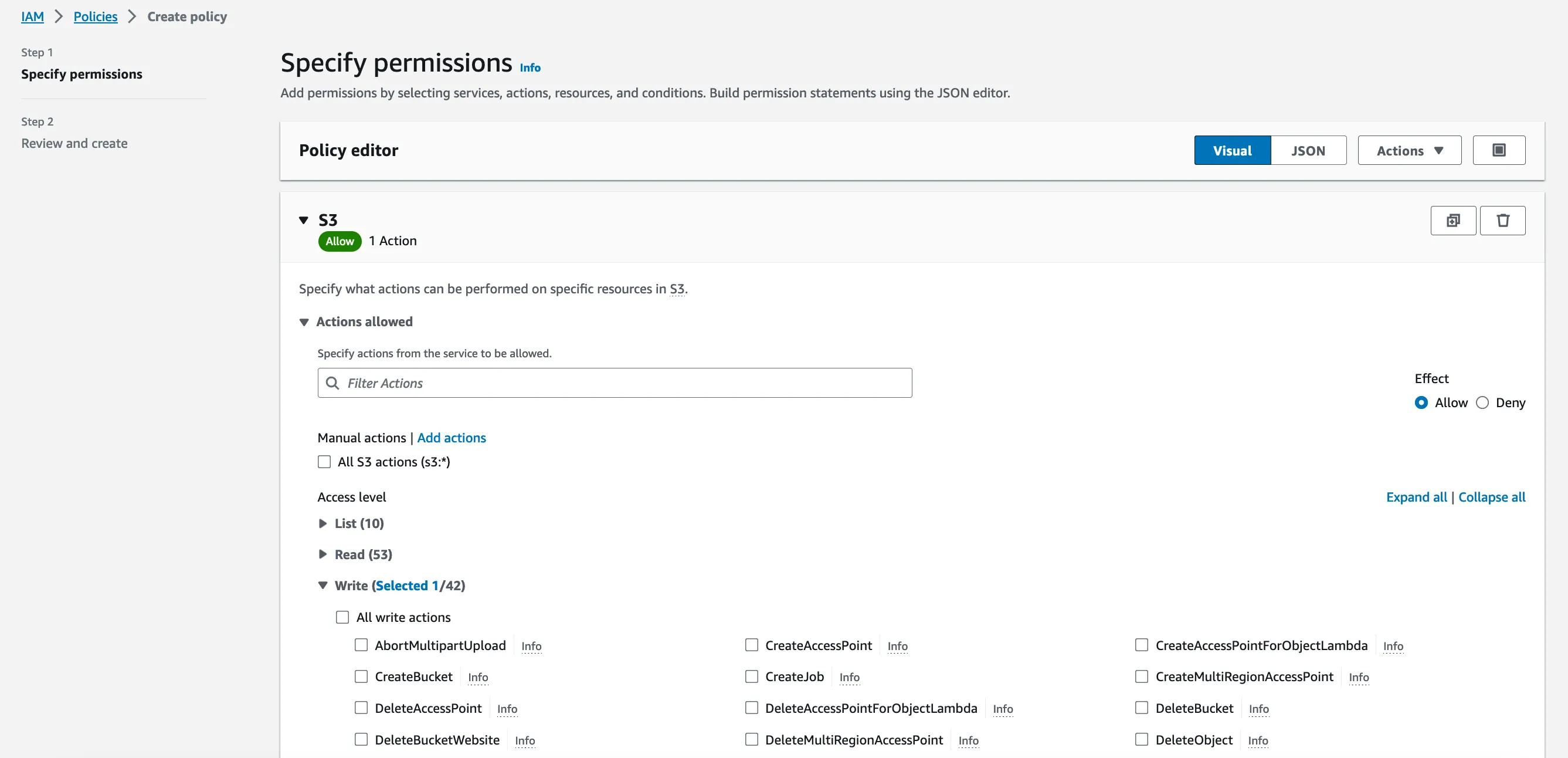
We just need one permission (s3:PutObject) on the contents of the bucket. The instance won’t have to read the files from there, so write permissions are sufficient.

Then we need to create an IAM role and associate it to the new IAM policy. Making it an EC2 role will automatically make it available as a potential instance profile when we go back to the EC2 console.

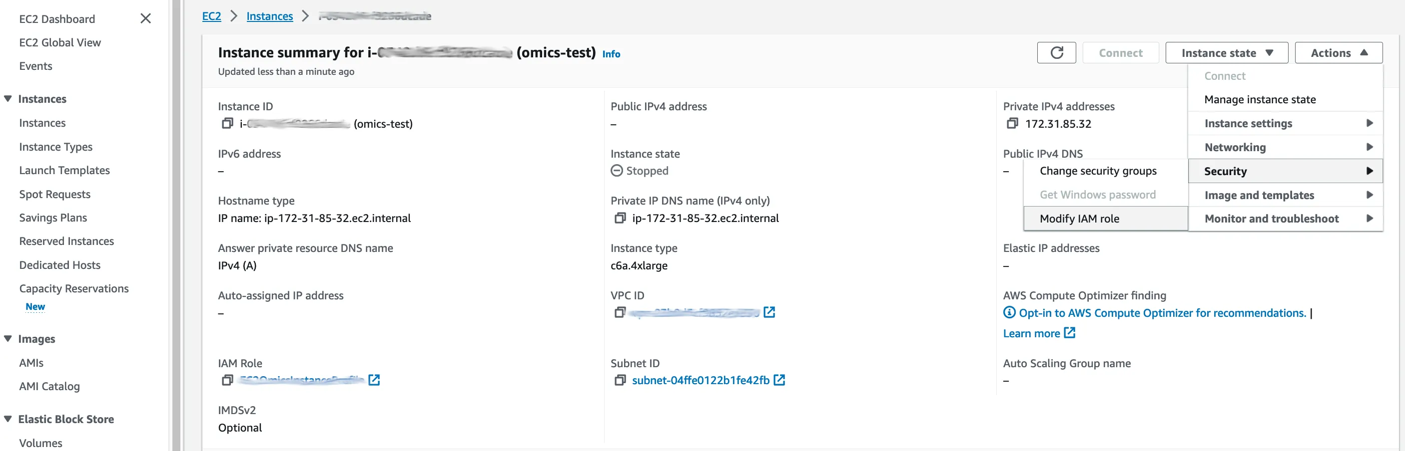
Back in the EC2 console, we select our instance, and in the ‘Action’ menu on the right, we select ‘Security’ > ‘Modify IAM role’.

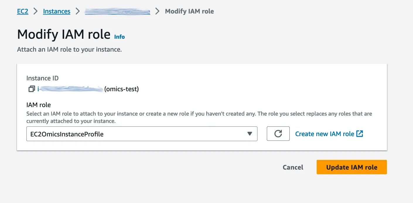
…our new role can be selected in a drop-down list. Hit ‘Update IAM role’ and our instance now has write access on the S3 bucket.

If that seems like a lot of work to get two AWS services talking together it’s a lot easier when you get the hang of it.

Also for a typical setup you would use Infrastructure as Code, scripting every in Terraform or the AWS CDK instead of using the AWS console. Now let’s publish our FastQC reports to the S3 bucket using the AWS CLI.

If we were on an Amazon Linux instance, the AWS CLI would be pre-installed. On our Ubuntu instance, we need to install it first.

sudo apt-get update
sudo apt-get install awscli

Now that the AWS CLI is installed, moving the FastQC reports to the S3 bucket is just two simple commands away.

Let’s write the to the following folder: ‘qc/thousand_genomes’.

aws s3 cp SRR038564_1.filt_fastqc.html s3://253601759346.omics.data/qc/thousand_genomes
aws s3 cp SRR038564_2.filt_fastqc.html s3://253601759346.omics.data/qc/thousand_genomes

Each S3 file has an associated url that you can open in your browser. You can find it by browsing to the file you want to open in the S3 console.

Visualizing the FastQC reports

Opening the FastQC report for the first of the two files, we find that the report includes some basic statistics about the dataset, as well as a number of graphs.

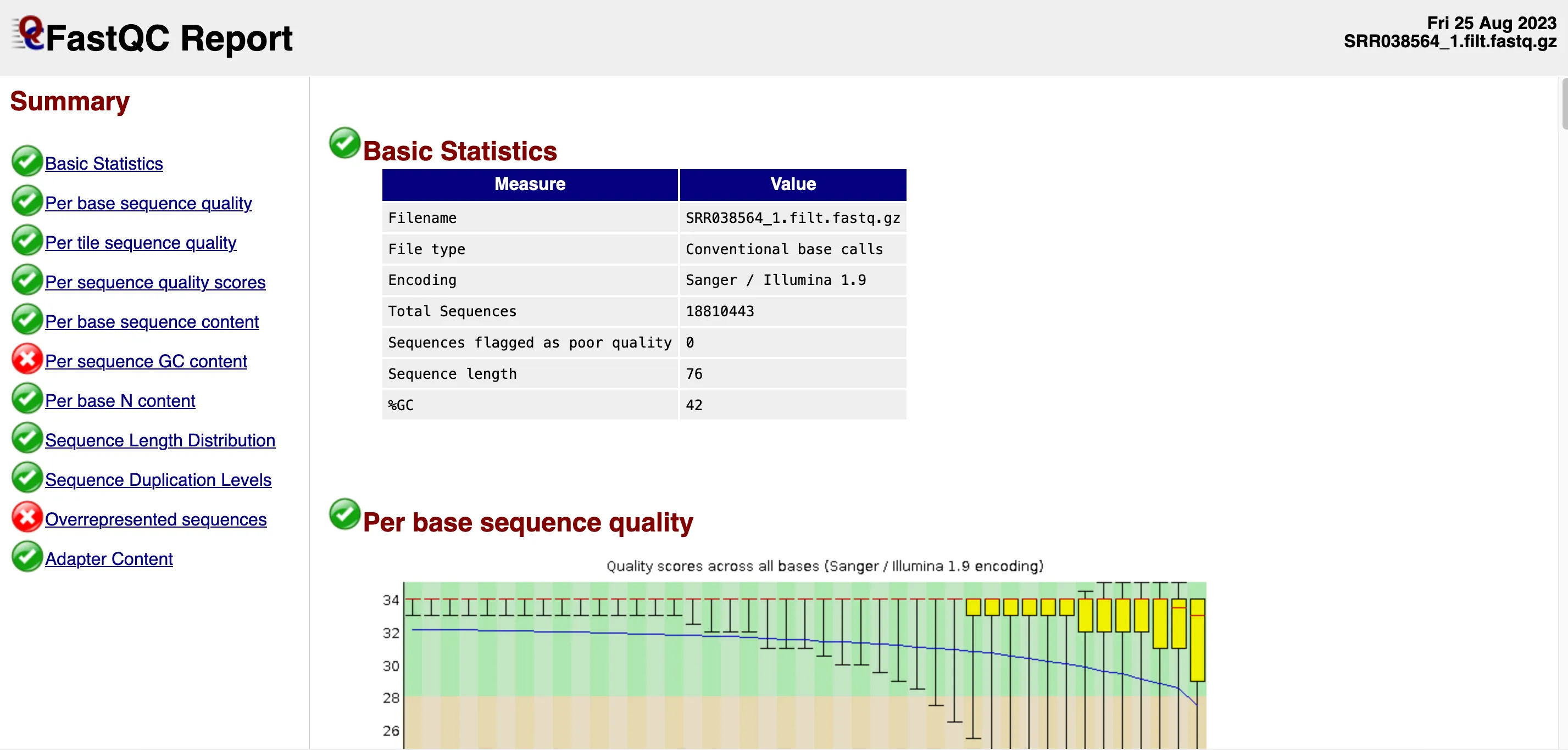
The Basic Statistics section confirms the size of the dataset as well as its encoding. No sequences have been flagged as poor quality which is a good sign.

Note the last two values in that table: read sequence length (76) and %GC (42). In this file, there are 18,810,443 sequences, each with 76 bases. That’s about 1.4 billion bases in total.

The human genome is estimated to be around 3.2 billion base pairs. However, sequencing 1.4 billion bases doesn’t mean we’ve covered 44% of all unique regions in the genome. In whole genome sequencing you typically aim for a multiple in terms of genome coverage in order to be able to do confident variant calling. %GC indicates the percentage of guanine (G) and cytosine (C) in a DNA sequence, relative to adenine (A) and thymine (T).

For most organisms, GC content is around 50%, while the human genome has an average GC content of 41%. The first graph titled “Per base sequence quality,” shows the confidence of base calls along the read.

Results are consistent with typical Illumina sequencing data. Initial quality is high but declines as confidence in base calls reduces. But as the yellow quartile rectangles on the right of the graph express, median quality is still decent in the latter part of each sequence.

GC content

Some bioinformatics workflows include a “trimming” step to keep only base calls with high Phred scores. Skipping ahead to the “Per base sequence content” graph, we get confirmation that A and T bases outnumber the G and C bases in a roughly 60-40 split.

This is consistent with the human genome as a whole, although some parts of the genome (like telomeres) are particularly AT-rich, while others are GC-rich.

In general exons (the coding regions of the genome) are relatively GC-richer than introns (the non-coding regions). Not all checks pass.

”Per sequence GC content” graph shows failure in FastQC. The graph compares observed and expected GC content distribution.

In this case, the red line differs significantly with two unexpected peaks. Possible explanation: The use of Epstein Barr Virus (EBV) to transform B lymphocytes into lymphoblastoid cell lines could explain the differences in GC content. Viral sequences may have been included in the genome, resulting in these discrepancies. The “Per base N content” graph indicates the absence of ambiguous bases.

A 0% “N” content implies that the base caller made a decision for each base, although not all decisions may be accurate. Bases with a lower Phred score are more likely to be incorrect.

Duplication

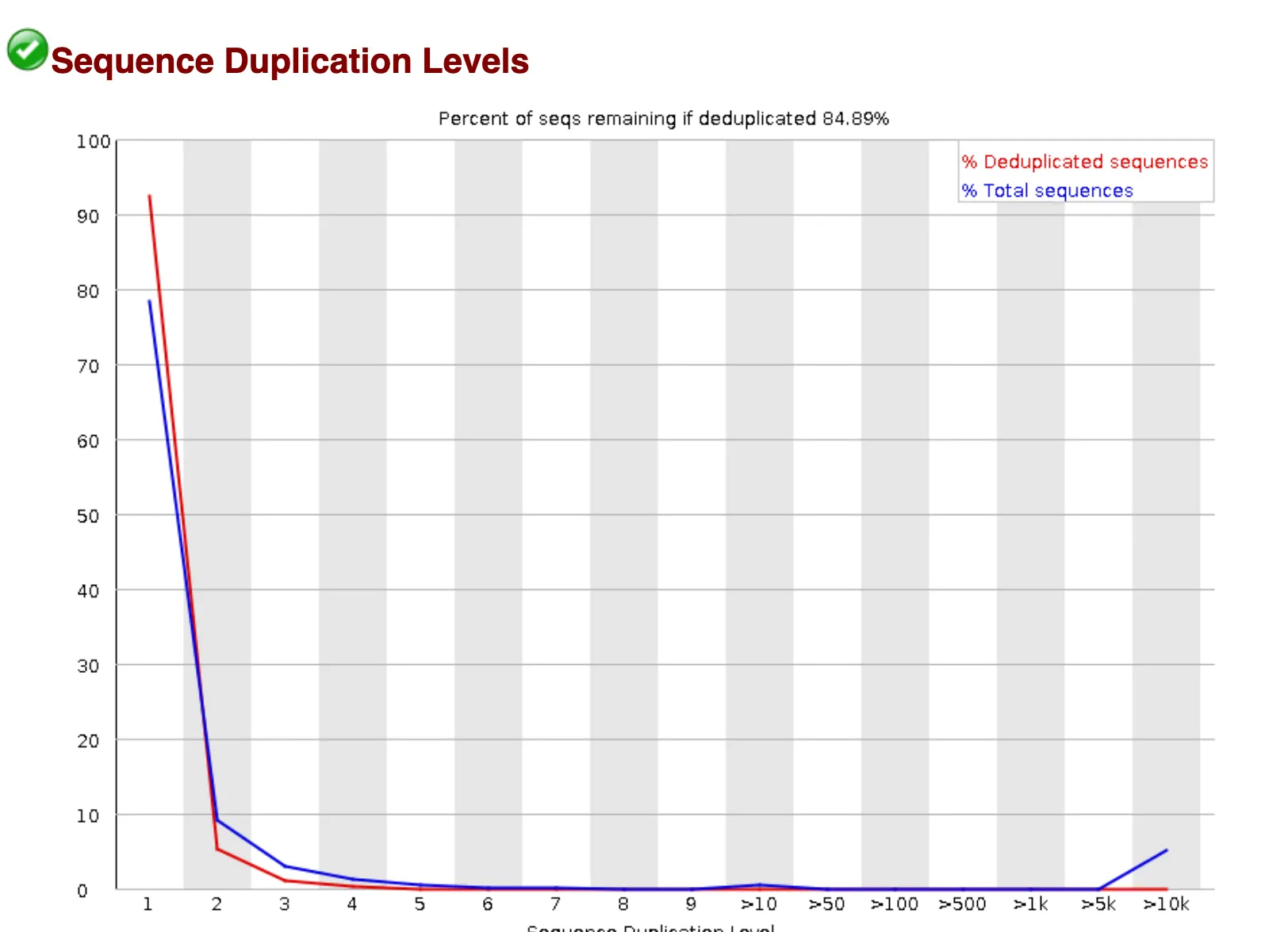
”Sequence Duplication Levels” graph:

Amplification and contamination can result in the duplication of certain sequences within the dataset. While most sequences appear only once, there is a small subset that appears thousands of times.

The FastQC report also flags the next check, “Overrepresented sequences” as failing. 4 sequences have found hundreds of thousands of times within the dataset.

The sequences below seem to appear repeatedly, making up as much as 1% of the entire dataset each.

There are a number of reasons why such sequences could be found in such numbers. A quick BLAST search against both the human and the EBV genomes does not yield any results, and as the next graph “Adapter content” shows there is no adapter content in the dataset.

Without knowing the library preparation details, it’s hard to understand what’s happening. Possibly contamination or PCR overamplification. One option is to remove overrepresented sequences and rerun FastQC. In our case, we’ll proceed with the analysis.

Reference genome

We have successfully sequenced the B lymphocyte cell line. Next step: compare to reference human genome, identify differences. The process includes genome alignment and variant calling.

We’ll start by downloading GRCh38 reference genome from the NCBI database (a gzipped FASTA file).

wget ftp://ftp.ncbi.nlm.nih.gov/genomes/all/GCA/000/001/405/GCA_000001405.15_GRCh38/seqs_for_alignment_pipelines.ucsc_ids/GCA_000001405.15_GRCh38_no_alt_analysis_set.fna.gz -O GRCh38_no_alt.fa.gz
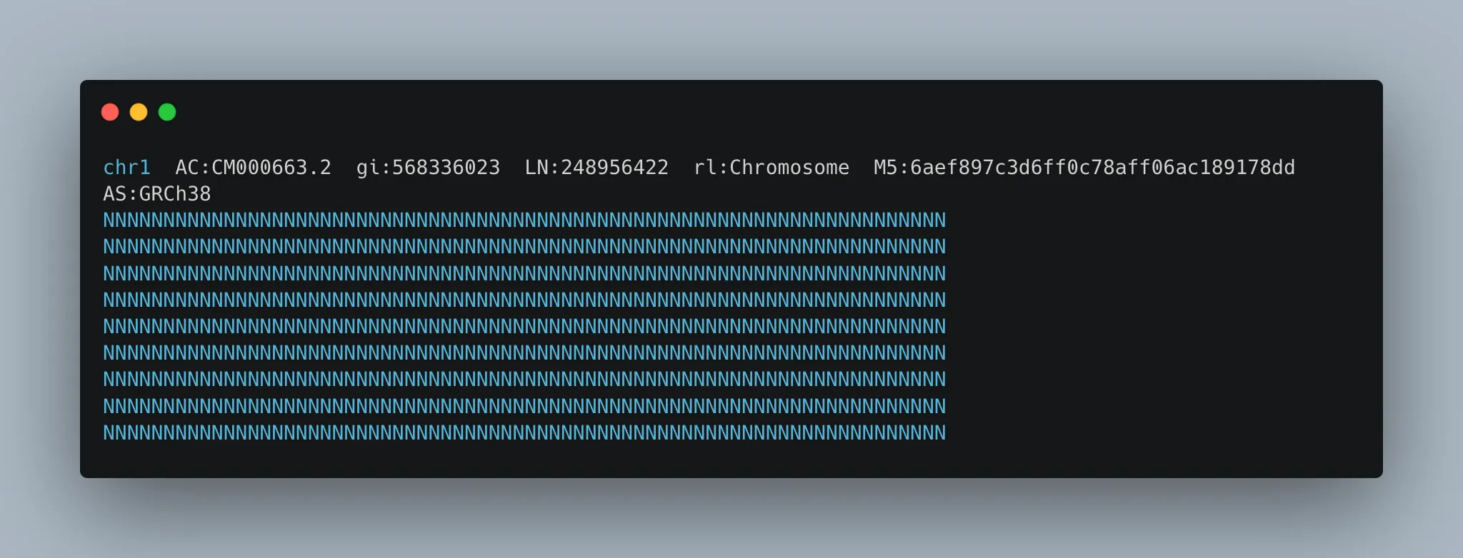
gunzip GRCh38_no_alt.fa.gz

To quickly check that we have a valid FASTA file, I ran ‘head GRCh38_no_alt.fa’ to see the FASTA header. It lists some metadata (chromosome name and length, etc).

The opening sequence is a series of ‘N’ values, indicating a region that could not be sequenced.

In order to do genome alignment, we first need to index the genome using the BWA tool. The index will be used as a kind of lookup table so that different parts of the genome can be quickly accessed during alignment.

Genome alignment

Each alignment tool uses a different indexation methods.

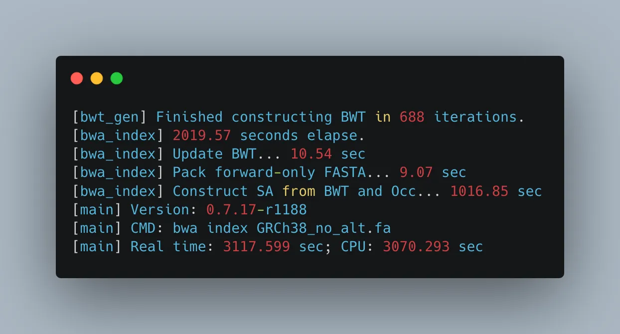
bwa index GRCh38_no_alt.fa

The indexation step is quite time-consuming. While it was processing, I used the ‘top’ command to monitor the performance of my EC2 instance.

Fortunately, the instance is comfortably underutilized, with only 6.2% of CPU usage and 4.7 GB of memory being utilized (out of 32). However, the ‘bwa’ command is consuming 99.7% of a CPU core (vCPU), indicating that the ‘bwa index’ operation is single-threaded. We have 16 vCPUs on our instance and only one of them was used in this longish computation. We could have used the ‘-b’ argument to specify a larger batch size for better performance but in this case the wait was bearable.

The indexing job has two parts: 1. BWA applies the Burrows-Wheeler Transform (BWT) algorithm to transform the genome, making string searches easier. 2. It then constructs the suffix array (SA), which is used in the alignment step. This is the part that takes long to complete.

With our indexed genome in place, we can now align our sequenced B lymphocyte dataset.

Notice that the ‘bwa mem’ command includes an ‘nproc’ argument. This means that the command will use the configured number of cores for parallel computation. We could replace this by a numeric value, but leaving it as-is will make bwa mem use all the cores at our disposal. This feature should speed up the process.

bwa mem -t `nproc` ./ncbi/GRCh38_no_alt.fa ./thousand_genomes/SRR038564_1.filt.fastq.gz ./thousand_genomes/SRR038564_2.filt.fastq.gz > SRR038564.bwa-mem.sam

Let’s run ‘top’ again as the alignment process unfolds.

This time we see that CPU usage is at 99.9% with 16 processes running so we are CPU-bound on this compute intensive EC2 instance. The alignment step justifies our choice of instance type!

In total the BWA-MEM alignment took about 34 seconds.

The output also informs us about insert size distribution and read orientation, but we won’t go into these detailed topics here.

We now have a SAM (Sequence Alignment/Map) file (SRR038564.bwa-mem.sam).

Post processing

Moving on to the post-processing steps, let’s compress the SAM file (into a BAM for Binary Alignment / Map) and we’re going to sort it to arrange the aligned reads by position in the reference genome.

samtools sort SRR038564.bwa-mem.sam > SRR038564.bwa-mem.sorted.bam

The resulting BAM file weighs in at about 2GB.

The next step is marking duplicates, thereby marking redundant reads due to amplification during sequencing. Duplicates can bias variant calling. To mark the duplicates we’re going to use a library called picard. It’s available in bioconda but I chose to download a Java archive (.jar file) and run it as a standalone Java program on my instance.

Before I could do this I first needed to install Java 17.

java -jar picard.jar MarkDuplicates I=SRR038564.bwa-mem.sorted.bam O=SRR038564.bwa-mem.sorted.marked.bam M=SRR038564.bwa-mem.sorted.marked.bam.metrics

The mark duplicates step takes about 5 minutes, and a new file has been generated: SRR038564.bwa-mem.sorted.marked.bam.

Now let’s index the BAM file so that we can rapidly access data from specific regions of the genome without scanning the entire file.

samtools index SRR038564.bwa-mem.sorted.marked.bam

The samtools index job runs quickly, generating a new file with a .bai extension that contains the index.

The following command is just a sanity check on the BAM file.

samtools flagstat SRR038564.bwa-mem.sorted.marked.bam

The output lists a number of statistics about the BAM file, including number of reads, number of reads mapped to the genome, and number of marked duplicate reads.

Variant calling

Next we’re going to do variant calling using the bcftools utility.

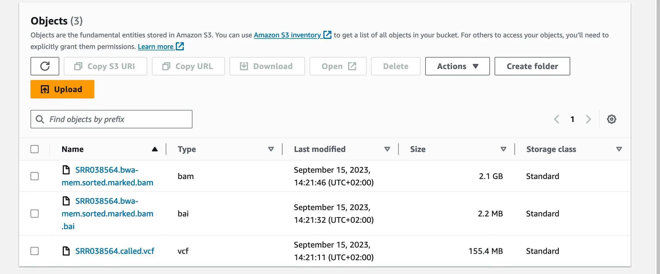
The resulting file is called “SRR038564.called.vcf” (VCF for Variant Calling File) and is about 160MB. The file should list all the variants identified in the sequence compared to the reference genome.

bcftools mpileup -Ou SRR038564.bwa-mem.sorted.marked.bam -f GRCh38_no_alt.fa --threads `nproc` | bcftools call --mv > SRR038564.called.vcf

Variants are genomic differences between the studied dataset and the expected nucleotide sequence in the reference genome, and come in various forms, from Single Nucleotide Polymorphisms (SNPs) and Indels to more complex variants. We’ve identified the variants in the B lymphocyte cell line. Now what insights can we glean form them?

Let’s start by counting the variants.

grep -v "^#" SRR038564.called.vcf | wc -l

We find a total of 1,466,521 variants of all types. This is within the expected range for an entire genome.

There may be false positives in there. One way to filter them out is to only count variants with a quality score of 20 or more. Let’s count them again.

bcftools view -i '%QUAL>=20' SRR038564.called.vcf | wc -l

This time there are only 281,310 left. This is a typical result. The remaining variants can be considered to be of high confidence.

Visualizing the variants

Finally we’re going to visualize the variants in the Integrated Genomics Viewer (IGV). The IGV is a visual tool developed by Broad Institute.

It enables to view your aligned reads, explore variants, and much more.

We’ll need to download the IGV (or use the web version).

Just like we did earlier with the FastQC report, we’re going to copy our BAM, BAI and VCF files from our EC2 instance into a new folder on our S3 bucket, and from there we’ll load the data into IGV.

I’ll be using the web version here. In IGV select the GRCh38 Human Genome under ‘Genome’ in the top menu. Then under ‘Tracks’, load the BAM and BAI files using their S3 urls.

Then go to the ‘Tracks’ menu again and this time enter the S3 url for the variant (VCF) file.

IGV shows two new tracks; one for the B lymphocyte sequence, and one for the variants. You can see that the data is arranged horizontally by chromosome, but at the default level of detail we don’t really see much at all. We need to start zooming in to see actual data.

We could start looking anywhere on the genome but since this is a female patient, let’s look for variants on or near the BRCA2 gene (associated with breast cancer on chromosome 13).

Here is what IGV shows when we zoom into one specific chromosome.

Let’s zoom even further. We know that BRCA2 is at position 13q13.1 (exact positions: 32,315,086 to 32,400,268 in the human genome). We want to zoom enough so that we can see the detail of the genome and the variant at the nucelotide level.

We can see an example of an SNP at position 32,354,180 in the region of BRCA2 (C instead of T). This does not mean that the patient has a predisposition for breast cancer. In fact this particular variant is in a non exonic region, so doesn’t directly code for proteins. Even introns can have an impact on disease profiling though. Establishing clinical relevance of this variant would involve searching through the ClinVar database or BRCA exchange. That’s a job for another day.

Conclusion

Running the entire pipeline on AWS should have cost me about $20. Most of this would be due to running a large EC2 instance. In reality it didn’t cost me anything at all because I have AWS credits that easily covered the expense.

This was of course just a brief foray into the world of bioinformatics. We’re going to go a lot deeper in upcoming threads. As a follow-up to this article, we’re going to perform a secondary analysis, delving deeper into the variants identified in this pipeline and trying to establish potential clinical relevance. Read all about this in our next piece!

What I love about the field is that it combines computational skills with biological research. It offers opportunities for software engineers to work with wet lab scientists.

I’m going to make the entire AWS setup available, including all libraries installed on the EC2 instance, AWS CLI, S3 buckets, reference genome and B lymphocyte files that you can just import into your own AWS account.

Let me know if there’s another bioinformatics topic that you’d like me to cover in my next series!